The Art of Slashing

class: center, middle, inverse, title-slide

# The Art of Slashing 
### Omni Analytics Group

---

## Case study

- Explore and perform analysis on a real dataset using R
- Goal: get good understanding of using R for data management, exploration, and analysis

## What is Ethereum?

Ethereum is a technology that lets you send cryptocurrency to anyone for a small fee. It also powers applications that everyone can use and no one can take down. It's the world's programmable blockchain and a marketplace of financial services, games and apps that can't steal your data or censor you.

Ethereum also has its own cryptocurrency, namely 'ETHER' or 'ETH' for short. Check out more about Ethereum and ETH on https://ethereum.org/.

---

## Slot-Slashed Dataset

This dataset is obtained from the Beacon Scan block explorer, where it provides the information on 1751 slashed validators. Being slashed means that a significant part of the validator’s stake is removed: up to the whole stake of 32 ETH in the worst case. Validator software and staking providers will have built-in protection against getting slashed accidentally. Slashing should only affect validators who misbehave deliberately. For more info, please visit https://codefi.consensys.net/blog/rewards-and-penalties-on-ethereum-20-phase-0.

## Why do validators get slashed?

Ethereum 2.0’s consensus mechanism has a couple of rules that are designed to prevent attacks on the network. Any validator found to have broken these rules will be slashed and ejected from the network. According to a blog post on Codefi, there are three ways a validator can gain the slashed condition:

1. By being a proposer and sign two different beacon blocks for the same slot.
2. By being an attester and sign an attestation that "surrounds" another one.
3. By being an attester and sign two different attestations having the same target.

---

## Explore the data in R

Let's load the data and look at the first few rows. Here, we will use the tidyverse package. We can use the sample_n() function to show n random rows.

```r
#load library
library(tidyverse)
#Load data
df_slashed <- read.csv("slot-slashed.csv") 
#Show 5 random rows of the data
sample_n(df_slashed,5)
```

```
##      X epoch   slot                age validatorSlashed slashedBy
## 1 1713  3250 104010 53 days 12 hrs ago             8122     13469
## 2  118 12567 402159  12 days 2 hrs ago            15378     36677
## 3  696  3352 107294   53 days 1 hr ago            24211     14561
## 4  303  7147 228714  36 days 4 hrs ago             2250     27206
## 5   71 13527 432876  7 days 20 hrs ago            38868     43676
##                     reason
## 1 Attestation rule offense
## 2 Attestation rule offense
## 3 Attestation rule offense
## 4 Attestation rule offense
## 5    Proposer rule offense
```

---

## The variables

The 7 variables are:

* `X` - The row index of the validator.
* `epoch` - The epoch number that the validator was slashed.
* `slot` - The slot number that the validator was slashed.
* `age` - The amount of time passed since the validator was slashed.
* `validatorSlashed` - The index of the validator who was slashed.
* `slashedBy` - The index of the validator who did the slashing.
* `reason` - The reason why the validator was slashed.

---
We begin our analysis with some high level statistics. Let's summarize the data using the skim() function from the skimr package. This command produces a simple summary table of centrality and spread statistics of our collected features.

```r
library(skimr)
skim(df_slashed)
```

.center[![summary1](images/summary1.PNG)]

---

We see that the data consists of 1751 rows, 2 character columns and 5 numeric columns.

Let's get the numbers of unique values in each column via summarise_all() and n_distinct .

```r
df_slashed %>% summarise_all(n_distinct)
```

```
##      X epoch slot age validatorSlashed slashedBy reason
## 1 1751   381  815 215             1647       771      2
```

--
Thus, we have 1647 unique validators that were slashed and they were slashed by 771 unique validators for only 2 reasons.

---

## Time series

Let's find out how many validators are slashed over time.

1. Sort the data by 'epoch' using arrange() 
2. Count the number of each 'epoch' group using group_by() and summarise(n())

```r
num_slashed <- df_slashed %>% 
 arrange(epoch) %>%
 group_by(epoch) %>% 
 summarise(count = n())
head(num_slashed)
```

```
## # A tibble: 6 x 2
## epoch count
## <int> <int>
## 1 4 1
## 2 21 1
## 3 39 1
## 4 477 1
## 5 530 1
## 6 918 2
```

---

We can plot a time series using geom_line from the ggplot2 package to see how the number changes over time.

.pull-left[

```r
num_slashed %>%
  ggplot(aes(x=epoch, y=count)) +
  scale_x_continuous(breaks = seq(0, 15000, by = 1000))+
  scale_y_continuous(breaks = seq(0, 150, by = 10))+
  geom_line()+
  labs(title="Number of slashed over epoch")
```
]

.pull-right[
![](2-1-Case-Study-Slashed_files/figure-html/p1-out-1.png)
]

---

To better assess the impact of these spikes in slashings, we produced a cumulative count plot that tracks the total number of slashings across epochs. We can do this very easily by simply adding a temporary column using mutate() and cumsum() .

.pull-left[

```r
num_slashed %>%
  mutate(cume_count = cumsum(count)) %>%
  ggplot(aes(x=epoch, y=cume_count)) +
  scale_x_continuous(breaks = seq(0, 15000, by = 1000))+
  scale_y_continuous(breaks = seq(0, 2000, by = 100))+
  geom_line()+
  labs(title="Number of slashed over epoch", y="Cumulative Frequency")
```

The first large spike in slashings occurs around epoch 3000 and another smaller spike in slashing around epoch 12500. Despite the fact that these jumps are significant, when focusing on the rate of change of slashings, the number of offensive rule violations are quite stable the majority of the time. Globally, the rate of slashing is approximately 117 slashes per 1000 epochs. When we exclude the spikes, the rate of change is approximately 63 slashes per 1000 epochs.

]

.pull-right[
![](2-1-Case-Study-Slashed_files/figure-html/p2-out-1.png)
]

---

## How much time elapsed between slashings?

Next, we can investigate how often a slash occurs. We need to take a few steps:

1. Create 'previousepoch' which is simply a 'epoch' shifted one row up 
2. Create 'epochelapsed' by subtracting 'previousepoch' from 'epoch'
3. Remove the rows where 'epochelapsed' is 0 by using filter() just to exclude slashings that occur within the same epoch.
4. Compute summary statistics

```r
Epochelapsed <- df_slashed %>% 
 mutate(previousepoch = c(tail(epoch,-1),0)) %>%
 mutate(epochelapsed = epoch - previousepoch) %>%
 filter(epochelapsed !=0)

Epochelapsed %>%
  summarise(
    min = min(epochelapsed),
    mean = mean(epochelapsed),
    max = max(epochelapsed))
```

```
##   min     mean max
## 1   1 39.59843 900
```

---

From the summary, we can see that approximately 40 epochs elapse between slashings on average, excluding slashings that occur in the same epoch. Let's plot the histogram so we can investigate further.

.pull-left[

```r
Epochelapsed %>%
  ggplot(aes(x=epochelapsed))+
  geom_histogram(color="darkblue", fill="lightblue",boundary=0)+
  labs(title="A Distribution of the Number of Epochs lapsed between Slashings", x="Epoch Elapsed", y="Frequency")+
  scale_y_continuous(breaks = seq(0, 300, by = 25))+
  scale_x_continuous(breaks = seq(0, 900, by = 50))
```
We can see that it is very common that less than 25 epochs will elapse between slashings. In fact, about 41% of the time only 1 epoch without a slashing will occur between two epochs with at least 1 slashing. The longest period without a slashing lasted 900 epochs, which is 93 hours.]

.pull-right[
![](2-1-Case-Study-Slashed_files/figure-html/p3-out-1.png)
]

---

## Your turn

We can find out more about the epoch elapsed between slashings.

1. Verify the fact that about 41% of the 'epochelapsed' is 1. 
2. Draw a red timeseries of 'epochelapsed' using 'previousepoch' and give it a title.

---

## Answer

### 1.

```r
Epochelapsed %>% 
  group_by(epochelapsed) %>%
  summarise(n = n()) %>% 
  mutate(percentage = n / sum(n)*100)
```

```
## # A tibble: 94 x 3
## epochelapsed n percentage
## <dbl> <int> <dbl>
## 1 1 156 40.9 
## 2 2 22 5.77 
## 3 3 17 4.46 
## 4 4 11 2.89 
## 5 5 10 2.62 
## 6 6 8 2.10 
## 7 7 13 3.41 
## 8 8 5 1.31 
## 9 9 3 0.787
## 10 10 2 0.525
## # ... with 84 more rows
```

---

### 2.

.pull-left[

```r
Epochelapsed %>%
  ggplot(aes(x=previousepoch,y=epochelapsed))+ geom_line(color="red")+
  labs(title = "Time series of epoch elapsed between slashings", x="Epoch", y = "Epoch Elapsed")+
  scale_y_continuous(breaks = seq(0, 1000, by = 100))+
  scale_x_continuous(breaks = seq(0, 16000, by = 1000))
```
]

.pull-right[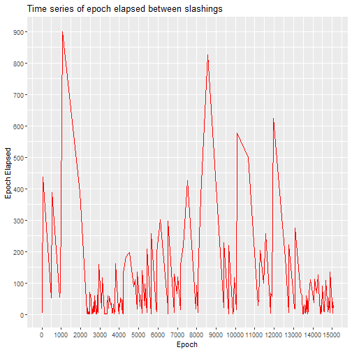
![](2-1-Case-Study-Slashed_files/figure-html/p4-out-1.png)
]
---

## Why are the validators slashed?

Of the three ways a validator can violate consensus rules, there are only two such categories of offenses: attestation rule and proposer rule violations. Let's create a histogram that shows the percentage of each reason why a validator was slashed.

One way to do it is similar to what we have been doing. we use group_by and summarise(n()) to get the data. Here, we can use geom_col() as we want to plot a bar chart as it is.

.pull-left[

```r
df_slashed %>%
  group_by(reason) %>%
  summarise(count= n()) %>%
  ggplot(aes(x=reason, y=count))+geom_col(width=0.5, fill="steelblue")+
  scale_y_continuous(breaks = scales::pretty_breaks(n=10))+
  labs(title="Number of slashes per reason")
```
We can also adjust the width and color as you can see here.]

.pull-right[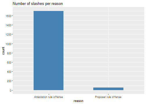
![](2-1-Case-Study-Slashed_files/figure-html/p5-out-1.png)
]

---

We can do it another way by only using ggplot2 package.

W will use geom_bar() here and we can use ..count.. for counting. Let's also add a label that shows the percentage of each reason using geom_text() and scales::percent() .

--
.pull-left[

```r
ggplot(df_slashed, aes(x= reason)) + 
 geom_bar(aes(y = ..count..),width=0.5, fill="steelblue") +
 geom_text(aes(label= scales::percent(..count../sum(..count..))), stat= "count", vjust = -0.25)+
 scale_y_continuous(breaks = scales::pretty_breaks(n=10))+
 labs(title="Number of slashes per reason")
```
Note that the we used vjust to adjust the position of the percentage label.]

.pull-right[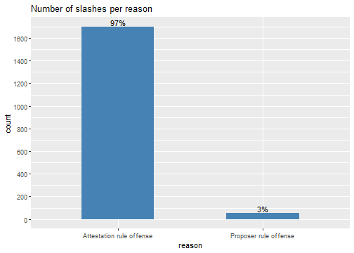
![](2-1-Case-Study-Slashed_files/figure-html/p6-out-1.png)
]

The distribution is skewed heavily towards attestation rule violations as they encompass nearly 97% of justifications for slashes in our data. The remaining 3% of slashes can be attributed to proposer rule offenses.

---

Interestingly, this distribution has not been constant over time. Let's find out exactly how it changes over time. To do so, we can do the following:

1. Convert 'reason' to factor
2. Group by 'epoch' and 'reason' 
3. Count each group using tally() (alternative function to summarise(n()) )

.pull-left[

```r
num_slashed_over_epoch_reason <- df_slashed %>%
 mutate(reason = factor(reason)) %>%
 group_by(epoch, reason, .drop = FALSE) %>%
 tally()
head(num_slashed_over_epoch_reason)
```
Notice that it is necessary for us to convert 'reason' to factor so that we can have 0 in our count, and to keep the 0, '.drop = FALSE' is needed. 
]

.pull-right[

```
## # A tibble: 6 x 3
## # Groups: epoch [3]
## epoch reason n
## <int> <fct> <int>
## 1 4 Attestation rule offense 0
## 2 4 Proposer rule offense 1
## 3 21 Attestation rule offense 1
## 4 21 Proposer rule offense 0
## 5 39 Attestation rule offense 1
## 6 39 Proposer rule offense 0
```
]

---

Now that we have the table, we can easily produce a time series of showing the numbers of the reason over time. Let's also use the facet_wrap() function to separate the time series by reason.

.pull-left[

```r
num_slashed_over_epoch_reason %>%
  ggplot(aes(x=epoch, y=n, group = reason, color =reason)) +
  geom_line() +
  labs(title="Reasons for slashes",x="epoch", y = "frequency")+
  facet_wrap(~reason)+
  theme(legend.position = "none")
```
]

.pull-right[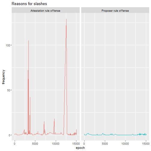
![](2-1-Case-Study-Slashed_files/figure-html/p7-out-1.png)
]

---
The plot is great but we can barely see the graph on the right as the frequency is dominated by the graph on the left. Let's fix that by using scales="free_y" so that each graph has its own y-scale.

.pull-left[

```r
ggplot(data=num_slashed_over_epoch_reason, aes(x=epoch, y=n, group = reason, color =reason)) +
  geom_line()+
  labs(title="Reasons for slashes",x="epoch", y = "frequency")+
  facet_wrap(~reason, scales="free_y") +
  theme(legend.position = "none")+
  scale_x_continuous(breaks = scales::pretty_breaks(n=10))+
  scale_y_continuous(breaks = scales::pretty_breaks(n=15))
```
Despite the proposer rule offenses being rare throughout all epochs it was, interestingly enough, the very first offense committed by a validator on the network. Overtime proposer violations have becoming more frequent as shown in the subsequent time series graphs.]

.pull-right[
![](2-1-Case-Study-Slashed_files/figure-html/p8-out-1.png)
]

---

## Your Turn

Create a time series of the cumulative number of the reason similar to the previous slide

Hint: you will need to use group_by() twice here.

---
## Answer

.pull-left[

```r
cumul_num_slashed_over_epoch_reason <- df_slashed %>%
 mutate(reason = factor(reason)) %>%
 group_by(epoch, reason, .drop = FALSE) %>%
 tally() %>%
 group_by(reason) %>%
 mutate(cumul = cumsum(n))

cumul_num_slashed_over_epoch_reason %>%
  ggplot(aes(x=epoch, y=cumul, group = reason, color=reason)) +
  geom_line()+
  labs(title="Reasons for slashes",x="epoch", y = "cummulative frequency")+
  theme(legend.position = "none")+
  facet_wrap(~reason,scales="free_y") +
  scale_x_continuous(breaks = scales::pretty_breaks(n=10))+
  scale_y_continuous(breaks = scales::pretty_breaks(n=20))
```
]

.pull-right[
![](2-1-Case-Study-Slashed_files/figure-html/p9-out-1.png)
]

---
## Slashed or Be Slashed

Let's turn our attention to the distribution of number of slashings received and the number of slashings performed.

.pull-left[
![](2-1-Case-Study-Slashed_files/figure-html/unnamed-chunk-7-1.png)
]

.pull-right[
![](2-1-Case-Study-Slashed_files/figure-html/unnamed-chunk-8-1.png)
]

---
## Your Turn

We can see that, of the validators that have slashed, most have only done slashings once or twice. Similarly, most validators, who have been slashed, have received only one or two lashings, and only a handful of them have been slashed more than 2 times.

Recreate those two plots on your own!

Hint: One uses geom_hist() and the other uses geom_bar() .

---

## Answers

FIrst plot:

```r
df_slashed %>% 
  group_by(slashedBy) %>% summarise(Freq = n()) %>%
  ggplot(aes(x=Freq)) + 
  geom_histogram(color="darkblue", fill="lightblue",boundary=0)+
  labs(title="Distribution of the Number of Slashings Performed by a Validator", x="Number of slashings", y="Frequency", subtitle = "For Validators with at least one slashing")+
  scale_x_continuous(breaks = seq(0, 100, by = 5))+
  scale_y_continuous(limits=c(0,750), breaks = seq(0, 750, by = 50))
```

Second plot:

```r
df_slashed %>% 
  group_by(validatorSlashed) %>% summarise(Freq = n()) %>%
  ggplot(aes(x=Freq)) + 
  geom_bar(color="darkblue", fill="lightblue")+
  labs(title="Distribution of the Number of Slashings Received by a Validator", y="Frequency",subtitle = "For Validators with at least one slashing")+
  scale_x_continuous(breaks = seq(1, 7, by = 1))+
  scale_y_continuous(breaks = seq(0, 1600, by = 100))
```

---

## Validator Data

To learn more about the validators, we will bring in a second dataset that is also obtained from the Beacon Scan block explorer. To learn more about the data set, you can read our case study on it as well. In short, this data set provides the following information on any given validator:

* `X` - The row index of the validator.
* `publickey` - The public key identifying the validator.
* `index` - The index number of the validator.
* `currentBalance` - The current balance, in ETH, of the validator.
* `effectiveBalance` - The effective balance, in ETH, of the validator.
* `proposed` - The number of blocks assigned, executed, and skipped by the validator.
* `eligibilityEpoch` - The epoch number that the validator became eligible.
* `activationEpoch` - The epoch number that the validator activated.
* `exitEpoch` - The epoch number that the validator exited.
* `withEpoch` - Epoch when the validator is eligible to withdraw their funds. This field is not applicable if the validator has not exited.
* `slashed` - Whether the given validator has been slashed.

---

## How long before a validator get slashed or slash others?

We have the 'epoch' when a validator was slashed and also their 'activationEpoch'. Thus, the difference will answer how long before a validator get slashed. However, we have some validators who was slashed more than once, we will need to get the rows where the first slashing occurs for each unique validator, i.e. the minimum difference.

However, 'epoch' and 'activationEpoch' are in different data set. Thus, we need to first combine these two datasets using the validator index. Since we want the 'activationEpoch' of the validator that was slashed, we will join the two tables on 'validatorSlashed' and 'index' via inner_join() .

Also, we need to convert 'activationEpoch' to numeric values.

```r
df_validator <- read.csv("validator_data.csv", header=T)
df_join_slashed <- df_slashed %>% 
 inner_join(df_validator, by = c("validatorSlashed"="index")) %>%
 mutate(SlashedActivation = as.numeric(ifelse(activationEpoch == "genesis", 0, activationEpoch)))
```

---

To find out how long before a validator get slashed, we will do the following:

1. Create 'timetoslashed' by subtracting 'SlashedActivation' from 'epoch' using mutate() 
2. Get the mininimum 'timetoslashed' of each group group_by and slice(which.min()) 
3. Use ungroup() to ungroup the data so we can compute summary statistics
4. Compute summary statistics using summarise()

.pull-left[

```r
df_join_slashed %>%
  mutate(timetoslashed = epoch - SlashedActivation) %>%
  group_by(validatorSlashed) %>%
  slice(which.min(timetoslashed)) %>%
  ungroup()%>%
  summarise(
    min = min(timetoslashed),
    mean = mean(timetoslashed),
    max = max(timetoslashed))
```
]

.pull-right[

```
## # A tibble: 1 x 3
## min mean max
## <dbl> <dbl> <dbl>
## 1 4 3919. 15087
```
]

---

Thus, on average, validators are slashed after 3919 epoch. Note that this average accounts for only validators who are slashed at least once. Similarly, we can compute 'timetoslash' to find out how long before a validator slashes others.

All we need to do is change a few things from the code in previous two slides. Take a few minutes to figure out the code!

```r
df_join_slasher <- df_slashed %>% 
 inner_join(df_validator, by = c("slashedBy"="index")) %>%
 mutate(SlasherActivation = as.numeric(ifelse(activationEpoch == "genesis", 0, activationEpoch)))
```

.pull-left[

```r
df_join_slasher %>%
  mutate(timetoslash = epoch - SlasherActivation) %>%
  group_by(slashedBy) %>%
  slice(which.min(timetoslash)) %>%
  ungroup()%>%
  summarise(
    min = min(timetoslash),
    mean = mean(timetoslash),
    max = max(timetoslash))
```
]

.pull-right[

```
## # A tibble: 1 x 3
## min mean max
## <dbl> <dbl> <dbl>
## 1 4 3409. 14892
```
On average, a validator marks their first slash in the initial 3409 epochs after activation. The fastest first slash was found to occur only 4 epochs after activation, while the slowest first slash was 14892 epochs after activation.]

---

## Top Slashers

In previous slide, we looked at the  Distribution of the Number of Slashings Performed by a Validator. There was a validator that has slashed others more than 90 times. We are interested to see who these frequent slashers are.

Since we have the data 'df_joined_slasher', we can easily get the information of these frequent slashers simply group by 'slashedBy' and arrange them according to their slashing frequency.

```r
df_join_slasher %>% 
  group_by(slashedBy) %>%
  mutate(SlashingFrequency=n()) %>%
  select(slashedBy, currentBalance, effectiveBalance, proposed, activationEpoch, SlashingFrequency) %>%
  distinct() %>%
  arrange(-SlashingFrequency) %>% head(10)
```

---

.center[![table1](images/table1.PNG)]

The table shows the top 10 validators that have done the most slashings. These slashers have similar current balance and effective balance. Most of them were also active for a long period of time. According to the tier system we created on the Case Study we did on validator data, 8 out of these top 10 slashers reside in tier 3 where validators' performance becomes noticeably worse.

---

## Visualizing the Slashings

Due to the sink-source structure of the 'slashedBy' and 'validatorSlashed' columns, it allows us to treat the various slashes as directed edges in a directed graph. A directed graph consists of a set of nodes and directed edges, where the directed edges represent some relationship between the nodes. The nodes in this instance are the individual validators, and a directed edge exists between two nodes if one node has slashed the other.

We will use the igraph package to draw the directed graph. We first need to get a dataframe using 'slashedBy' and 'validatorSlashed'. Then, we use graph_from_data_frame() to get a network object that we can then plot.

```r
library(igraph)
networkData <- data.frame(df_slashed$slashedBy,df_slashed$validatorSlashed)
network <- graph_from_data_frame(networkData) 
plot(network,layout=layout.sphere(network),vertex.size=2, edge.arrow.size=0.01, vertex.label=NA, main="Whole network")
```

Note that the order matters when we created the dataframe as we want the directed edge to point at 'validatorSlashed'. As you can see, we can customize how the graph looks with various parameters.

---

.center[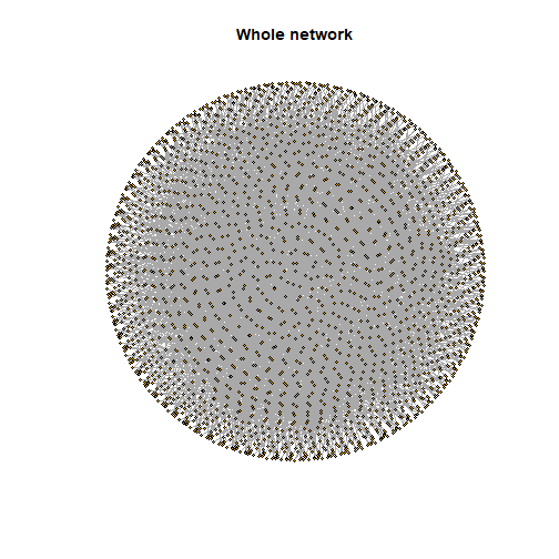
![](2-1-Case-Study-Slashed_files/figure-html/p10-out-1.png)
]

---

Since the whole network comprised of many vertices, we can decompose the network to all its connected subgraphs to have a better understanding using decompose.graph() .

.pull-left[

```r
dnetwork <- decompose.graph(network)
length(dnetwork)
```
]

.pull-right[

```
## [1] 660
```
]

We see that there are a total of 660 connected subgraphs.

---

To plot any of these subgraphs, we can simply use the following code:

```r
#plotting the first subgraph
plot(dnetwork[[1]])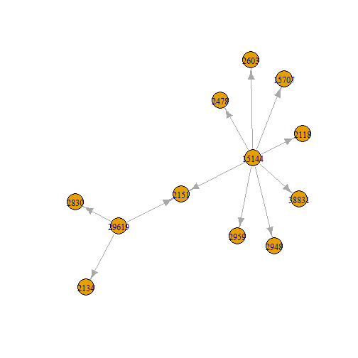
```

![](2-1-Case-Study-Slashed_files/figure-html/unnamed-chunk-14-1.png)

---
Let's find the subgraphs with the highest numbers of vertices. To do so, we can simply use a for loop and vcount() to count the number of vertices of each subgraph.

```r
num_vertices <-(1:length(dnetwork))*0 #create a vector of length 660 containing zeroes
for (i in 1:length(dnetwork)){
 num_vertices[i] <- vcount(dnetwork[[i]])
}

which.max(num_vertices)
```

```
## [1] 86
```

```r
max(num_vertices)
```

```
## [1] 415
```
--

Thus, the 86th subgraph has the 415 vertices, the highest number of vertices.

---

Here is the plot of the largest connected subgraph (86th subgraph).

```r
plot(dnetwork[[86]],layout=layout.davidson.harel(dnetwork[[86]]),vertex.size=5, edge.arrow.size=0.3, vertex.label=NA, main="415 vertices")
```

.pull-left[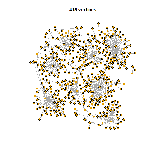
![](2-1-Case-Study-Slashed_files/figure-html/p11-out-1.png)
]

.pull-right[

we can see 8 validators that have done a high number of slashes and each of them have a star structure as they never slash the same validator twice.

]

---

## Your turn

1. Find the second largest connected subgraph and its number of vertices.
2. Plot the second largest connected subgraph

Hint: use sort() and which()

---

## Answers

###1.

```r
sort(num_vertices, decreasing=TRUE)[2]
```

```
## [1] 155
```

```r
which(num_vertices==155)
```

```
## [1] 70
```
So, the 70th subgraph is the second largest connected subgraph and it has 155 vertices.

---

###2

```r
plot(dnetwork[[70]],layout=layout.davidson.harel(dnetwork[[70]]),vertex.size=5, edge.arrow.size=0.4, vertex.label=NA, main="155 vertices")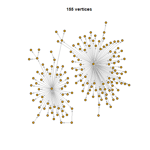
```

![](2-1-Case-Study-Slashed_files/figure-html/unnamed-chunk-17-1.png)

---

## Interesting observations

There were two interesting observations about the slashing behavior that were particularly important to understanding the nature of the network visualizations.

The first was that there was not one validator that had been slashed by the same validator twice.

The second observation we discovered was that there were no instances of "revenge slashing" in which a validator slashed a second validator, and then the second validator eventually slashed the first in return.

When you combine these two facts, it explains why all of the networks we produced were only simple directed graphs (i.e. it has no loops or multiple edges).

---

## Conclusion
Through our analysis of ETH2's security mechanism for blockchain security known as "slashing", we've observed some interesting patterns in its frequency, those who perform them, and their recipients. Some key findings include:

* Less than 1% of the validators have been slashed or slashed someone else.
* The number of attestation offenses vastly outweighed the number of proposer rule violations.
* Slashings take place at a rate of only 6.3 per 100 epochs.
* We identified presence of "super-slashers" who, despite their prevalence for slashing other validators, typically  didn't have the best performance themselves.
* There was no evidence of "revenge" slashing, where a validator who was slashed reciprocated one.
* No two pairs of slasher and slashed appeared twice in the data.
* Slashing patterns in the network induce a simple star like structure when graphing the nodes and edges,
* Complexity in the graphs come in the form of single link or multi link connections that expand with the number of slashings.

As the network of interconnected violators continues to grow, we expect the number of interesting sub-graphs to grow with it and represent some interesting dynamics in terms of the interaction between validators as it pertains to slashing.

---

## References

* Ethereum [https://ethereum.org/]
* Medalla Data Challenge [https://ethereum.org/en/eth2/get-involved/medalla-data-challenge/]
* Medalla Data Challenge Wishlist [https://www.notion.so/Wishlist-The-Eth2-Medalla-Data-Challenge-69fe10ffe83748bc87faa0e2586ba857]
* Ethereum 2.0 Beacon Chain Explorer [beaconscan.com/]
* Consensys Glossary of Ethereum 2.0 Terms [https://consensys.net/knowledge-base/ethereum-2/glossary/]
* Breaking Down ETH 2.0 - Sharding Explained [https://academy.ivanontech.com/blog/breaking-down-eth-2-0-sharding-explained]
* Rewards and Penalties on Ethereum 2.0 [Phase 0] [https://codefi.consensys.net/blog/rewards-and-penalties-on-ethereum-20-phase-0]
* Ethereum 2.0 Explained | Part II | Phase 0 and the Beacon Chain [https://youtu.be/-qwSAFcicg8]